N-HITS Forecasting with Nixtla’s NeuralForecast

Dataset: KaggleWPGD

This notebook demonstrates how to use the N-HITS forecasting model described in:

N-HiTS: Neural Hierarchical Interpolation for Time Series Forecasting, https://arxiv.org/abs/2201.12886

The implementation we use is provided by Nixtla’s NeuralForecast library:

for the base model NHITS
for the automodel AutoNHITS

Important note:

This notebook uses the following conda environments:

Under linux: tfm_cc, described in the tfm_cc.yml file (see environments folder).
Under macOS: tfm_cc_nixtla, described in the tfm_cc_nixtla.yml file (see environments folder).

Execution Notes:

The run times that appear below correspond to the execution of the notebook in a Linux machine under Ubuntu 22.04 LTS with Intel Core i7-10870H CPU (2.20GHz), 64GB of RAM, NVIDIA GeForce RTX 3060 Laptop GPU with 6Gb VRAM.

Load basic libraries

Warning: Model specific libraries will be loaded below.

import pandas as pd
import numpy as np
import matplotlib.pyplot as plt

import time
import logging



from sklearn.preprocessing import MinMaxScaler
from sklearn.preprocessing import StandardScaler
from sklearn.model_selection import train_test_split
from sklearn.metrics import mean_absolute_error

Load dataset

The data in this notebook comes from the Kaggle dataset:

Wind Power Generation Data - Forecasting

file_path = "../../data/kaggleWPGD/Location1.csv"
df = pd.read_csv(file_path, delimiter=',')
df.head()

	Time	temperature_2m	relativehumidity_2m	dewpoint_2m	windspeed_10m	windspeed_100m	winddirection_10m	winddirection_100m	windgusts_10m	Power
0	2017-01-02 00:00:00	28.5	85	24.5	1.44	1.26	146	162	1.4	0.1635
1	2017-01-02 01:00:00	28.4	86	24.7	2.06	3.99	151	158	4.4	0.1424
2	2017-01-02 02:00:00	26.8	91	24.5	1.30	2.78	148	150	3.2	0.1214
3	2017-01-02 03:00:00	27.4	88	24.3	1.30	2.69	58	105	1.6	0.1003
4	2017-01-02 04:00:00	27.3	88	24.1	2.47	4.43	58	84	4.0	0.0793

Set datetime format and index

df['time'] = pd.to_datetime(df['Time'], format='%Y-%m-%d %H:%M:00')
df.drop(columns=['Time'], inplace=True)
df.set_index('time', inplace=True)
df.head()

	temperature_2m	relativehumidity_2m	dewpoint_2m	windspeed_10m	windspeed_100m	winddirection_10m	winddirection_100m	windgusts_10m	Power
time
2017-01-02 00:00:00	28.5	85	24.5	1.44	1.26	146	162	1.4	0.1635
2017-01-02 01:00:00	28.4	86	24.7	2.06	3.99	151	158	4.4	0.1424
2017-01-02 02:00:00	26.8	91	24.5	1.30	2.78	148	150	3.2	0.1214
2017-01-02 03:00:00	27.4	88	24.3	1.30	2.69	58	105	1.6	0.1003
2017-01-02 04:00:00	27.3	88	24.1	2.47	4.43	58	84	4.0	0.0793

df.info()

<class 'pandas.core.frame.DataFrame'>
DatetimeIndex: 43800 entries, 2017-01-02 00:00:00 to 2021-12-31 23:00:00
Data columns (total 9 columns):
 #   Column               Non-Null Count  Dtype  
---  ------               --------------  -----  
 0   temperature_2m       43800 non-null  float64
 1   relativehumidity_2m  43800 non-null  int64  
 2   dewpoint_2m          43800 non-null  float64
 3   windspeed_10m        43800 non-null  float64
 4   windspeed_100m       43800 non-null  float64
 5   winddirection_10m    43800 non-null  int64  
 6   winddirection_100m   43800 non-null  int64  
 7   windgusts_10m        43800 non-null  float64
 8   Power                43800 non-null  float64
dtypes: float64(6), int64(3)
memory usage: 3.3 MB

Select a subset of the data

df = df.head(7248)

Rename the columns

initial_columns = df.columns.tolist()
initial_columns

['temperature_2m',
 'relativehumidity_2m',
 'dewpoint_2m',
 'windspeed_10m',
 'windspeed_100m',
 'winddirection_10m',
 'winddirection_100m',
 'windgusts_10m',
 'Power']

df.rename(columns={'Power' : 'Active_Power', 'windspeed_10m' : 'Wind_speed_tower'}, inplace=True)
df = df[['Active_Power', 'Wind_speed_tower']]
df

	Active_Power	Wind_speed_tower
time
2017-01-02 00:00:00	0.1635	1.44
2017-01-02 01:00:00	0.1424	2.06
2017-01-02 02:00:00	0.1214	1.30
2017-01-02 03:00:00	0.1003	1.30
2017-01-02 04:00:00	0.0793	2.47
...	...	...
2017-10-30 19:00:00	0.6847	5.89
2017-10-30 20:00:00	0.6841	6.32
2017-10-30 21:00:00	0.6834	6.52
2017-10-30 22:00:00	0.6828	6.33
2017-10-30 23:00:00	0.6822	6.15

7248 rows × 2 columns

Check for missing values and duplicated dates

There are no missing data in this dataset

print(df.isna().sum())

Active_Power        0
Wind_speed_tower    0
dtype: int64

duplicate_dates = df.index[df.index.duplicated(keep='first')]
print(f"Number of duplicate timestamps: {len(duplicate_dates)}")
print(duplicate_dates)

Number of duplicate timestamps: 0
DatetimeIndex([], dtype='datetime64[ns]', name='time', freq=None)

expected = pd.date_range(start=df.index.min(), end=df.index.max(), freq='h')
missing = expected.difference(df.index)
print("Missing timestamps:", missing)

Missing timestamps: DatetimeIndex([], dtype='datetime64[ns]', freq='h')

missing_df = pd.DataFrame({'missing':missing})
missing_df['date'] = missing_df['missing'].dt.date
missing_df.value_counts('date').sort_index()

Series([], Name: count, dtype: int64)

Target and exogenous variables

target = 'Active_Power'

features = [col for col in df.columns if col != target]
features = features[:1]
features

['Wind_speed_tower']

df = df[features + [target]]
df

	Wind_speed_tower	Active_Power
time
2017-01-02 00:00:00	1.44	0.1635
2017-01-02 01:00:00	2.06	0.1424
2017-01-02 02:00:00	1.30	0.1214
2017-01-02 03:00:00	1.30	0.1003
2017-01-02 04:00:00	2.47	0.0793
...	...	...
2017-10-30 19:00:00	5.89	0.6847
2017-10-30 20:00:00	6.32	0.6841
2017-10-30 21:00:00	6.52	0.6834
2017-10-30 22:00:00	6.33	0.6828
2017-10-30 23:00:00	6.15	0.6822

7248 rows × 2 columns

Train / Validation / Test split

We select the following lengths for the train, validation, and test sets:

int(np.ceil(df.shape[0] * 0.8))

train_len = 5800 # approx int(np.ceil(df.shape[0] * 0.8))
print(f"Train length: {train_len}")

val_len = (df.shape[0] - train_len) // 2
print(f"Validation length: {val_len}")

test_len = df.shape[0] - train_len - val_len
print(f"Test length: {test_len}")

Train length: 5800
Validation length: 724
Test length: 724

And we split the time series into train, validation, and test sets:

train_df = df.iloc[:train_len]
train_df

	Wind_speed_tower	Active_Power
time
2017-01-02 00:00:00	1.44	0.1635
2017-01-02 01:00:00	2.06	0.1424
2017-01-02 02:00:00	1.30	0.1214
2017-01-02 03:00:00	1.30	0.1003
2017-01-02 04:00:00	2.47	0.0793
...	...	...
2017-08-31 11:00:00	4.83	0.6155
2017-08-31 12:00:00	5.15	0.5935
2017-08-31 13:00:00	5.47	0.5536
2017-08-31 14:00:00	5.61	0.5137
2017-08-31 15:00:00	5.79	0.4738

5800 rows × 2 columns

val_df = df.iloc[train_len:(train_len + val_len)]
val_df

	Wind_speed_tower	Active_Power
time
2017-08-31 16:00:00	5.87	0.4339
2017-08-31 17:00:00	5.19	0.3940
2017-08-31 18:00:00	4.26	0.3605
2017-08-31 19:00:00	2.21	0.3334
2017-08-31 20:00:00	2.55	0.3063
...	...	...
2017-09-30 15:00:00	2.12	0.0907
2017-09-30 16:00:00	2.42	0.0991
2017-09-30 17:00:00	2.10	0.1076
2017-09-30 18:00:00	2.20	0.1166
2017-09-30 19:00:00	1.97	0.1262

724 rows × 2 columns

test_df = df.iloc[(train_len + val_len):]
test_df

	Wind_speed_tower	Active_Power
time
2017-09-30 20:00:00	1.80	0.1357
2017-09-30 21:00:00	1.71	0.1453
2017-09-30 22:00:00	1.44	0.1548
2017-09-30 23:00:00	1.40	0.1644
2017-10-01 00:00:00	2.20	0.1739
...	...	...
2017-10-30 19:00:00	5.89	0.6847
2017-10-30 20:00:00	6.32	0.6841
2017-10-30 21:00:00	6.52	0.6834
2017-10-30 22:00:00	6.33	0.6828
2017-10-30 23:00:00	6.15	0.6822

724 rows × 2 columns

Time series split visualization

plt.figure(figsize=(16, 6))
plt.plot(train_df["Active_Power"], label="Training Data", color='blue')
plt.plot(val_df["Active_Power"], label="Validation Data", color='green')
plt.plot(test_df["Active_Power"], label="Test Data", color='red')
plt.title("Active Power Time Series")
plt.xlabel("Time")
plt.ylabel("Active Power")
plt.legend(fontsize='small')

<matplotlib.legend.Legend at 0x73baf6c55a20>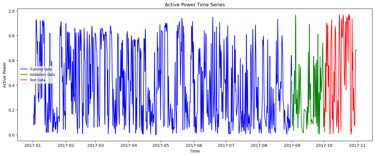

plt.figure(figsize=(16, 6))
plt.plot(train_df["Active_Power"].head(960), label="Training Data", color='blue')
# plt.plot(val_df["Active_Power"].head(240), label="Validation Data", color='green')
# plt.plot(test_df["Active_Power"], label="Test Data", color='red')
plt.title("Active Power Time Series")
plt.xlabel("Time")
plt.ylabel("Active Power")
plt.legend(fontsize='small')

<matplotlib.legend.Legend at 0x73baf631bfa0>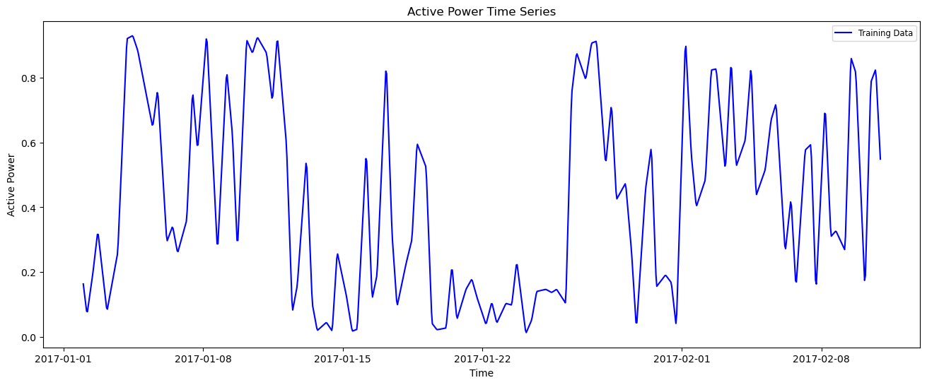

We will also create copies of the train, validation, and test sets to use them later in the notebook.

train_df_original = train_df.copy()
val_df_original = val_df.copy()
test_df_original = test_df.copy()

Data scaling

We apply the min-max scaler fitted to the training set to the train, validation, and test sets (to avoid data leakage).

from sklearn.preprocessing import MinMaxScaler

scaler = MinMaxScaler()
scaler.set_output(transform='pandas')

scaler.fit(train_df)
train_df = scaler.transform(train_df)

val_df = scaler.transform(val_df)
test_df = scaler.transform(test_df)

Let us check the result

train_df.describe().transpose()

	count	mean	std	min	25%	50%	75%	max
Wind_speed_tower	5800.0	0.275745	0.127310	0.0	0.184488	0.249247	0.348645	1.0
Active_Power	5800.0	0.407862	0.287194	0.0	0.149394	0.349394	0.669188	1.0

Nixtla Dataset Format

Convert to NeuralForecast format (ds, y, unique_id)



train_df_nf = train_df.copy()
train_df_nf = train_df_nf.rename(columns={target: 'y'})
train_df_nf['ds'] = train_df_nf.index

train_df_nf['unique_id'] = 'series_1'

Move ds and unique_id to front


train_df_nf = train_df_nf[['unique_id', 'ds', 'y'] + features]
train_df_nf

	unique_id	ds	y	Wind_speed_tower
time
2017-01-02 00:00:00	series_1	2017-01-02 00:00:00	0.172377	0.108434
2017-01-02 01:00:00	series_1	2017-01-02 01:00:00	0.150132	0.155120
2017-01-02 02:00:00	series_1	2017-01-02 02:00:00	0.127992	0.097892
2017-01-02 03:00:00	series_1	2017-01-02 03:00:00	0.105746	0.097892
2017-01-02 04:00:00	series_1	2017-01-02 04:00:00	0.083606	0.185994
...	...	...	...	...
2017-08-31 11:00:00	series_1	2017-08-31 11:00:00	0.648919	0.363705
2017-08-31 12:00:00	series_1	2017-08-31 12:00:00	0.625725	0.387801
2017-08-31 13:00:00	series_1	2017-08-31 13:00:00	0.583658	0.411898
2017-08-31 14:00:00	series_1	2017-08-31 14:00:00	0.541592	0.422440
2017-08-31 15:00:00	series_1	2017-08-31 15:00:00	0.499526	0.435994

5800 rows × 4 columns

Same for validation and test sets

val_df_nf = val_df.copy()
val_df_nf = val_df_nf.rename(columns={target: 'y'})
val_df_nf['ds'] = val_df_nf.index

val_df_nf['unique_id'] = 'series_1'

val_df_nf = val_df_nf[['unique_id', 'ds', 'y'] + features]
val_df_nf

	unique_id	ds	y	Wind_speed_tower
time
2017-08-31 16:00:00	series_1	2017-08-31 16:00:00	0.457459	0.442018
2017-08-31 17:00:00	series_1	2017-08-31 17:00:00	0.415393	0.390813
2017-08-31 18:00:00	series_1	2017-08-31 18:00:00	0.380074	0.320783
2017-08-31 19:00:00	series_1	2017-08-31 19:00:00	0.351502	0.166416
2017-08-31 20:00:00	series_1	2017-08-31 20:00:00	0.322931	0.192018
...	...	...	...	...
2017-09-30 15:00:00	series_1	2017-09-30 15:00:00	0.095625	0.159639
2017-09-30 16:00:00	series_1	2017-09-30 16:00:00	0.104481	0.182229
2017-09-30 17:00:00	series_1	2017-09-30 17:00:00	0.113442	0.158133
2017-09-30 18:00:00	series_1	2017-09-30 18:00:00	0.122931	0.165663
2017-09-30 19:00:00	series_1	2017-09-30 19:00:00	0.133052	0.148343

724 rows × 4 columns

test_df_nf = test_df.copy()
test_df_nf = test_df_nf.rename(columns={target: 'y'})
test_df_nf['ds'] = test_df_nf.index

test_df_nf['unique_id'] = 'series_1'

test_df_nf = test_df_nf[['unique_id', 'ds', 'y'] + features]
test_df_nf

	unique_id	ds	y	Wind_speed_tower
time
2017-09-30 20:00:00	series_1	2017-09-30 20:00:00	0.143068	0.135542
2017-09-30 21:00:00	series_1	2017-09-30 21:00:00	0.153189	0.128765
2017-09-30 22:00:00	series_1	2017-09-30 22:00:00	0.163205	0.108434
2017-09-30 23:00:00	series_1	2017-09-30 23:00:00	0.173326	0.105422
2017-10-01 00:00:00	series_1	2017-10-01 00:00:00	0.183342	0.165663
...	...	...	...	...
2017-10-30 19:00:00	series_1	2017-10-30 19:00:00	0.721877	0.443524
2017-10-30 20:00:00	series_1	2017-10-30 20:00:00	0.721244	0.475904
2017-10-30 21:00:00	series_1	2017-10-30 21:00:00	0.720506	0.490964
2017-10-30 22:00:00	series_1	2017-10-30 22:00:00	0.719873	0.476657
2017-10-30 23:00:00	series_1	2017-10-30 23:00:00	0.719241	0.463102

724 rows × 4 columns

Create a joint dataset with train and validation to fit into Nixtla’s framework.

train_val_df = pd.concat([train_df_nf, val_df_nf], axis=0)
train_val_df.reset_index(drop=True, inplace=True)
train_val_df.info()

<class 'pandas.core.frame.DataFrame'>
RangeIndex: 6524 entries, 0 to 6523
Data columns (total 4 columns):
 #   Column            Non-Null Count  Dtype         
---  ------            --------------  -----         
 0   unique_id         6524 non-null   object        
 1   ds                6524 non-null   datetime64[ns]
 2   y                 6524 non-null   float64       
 3   Wind_speed_tower  6524 non-null   float64       
dtypes: datetime64[ns](1), float64(2), object(1)
memory usage: 204.0+ KB

And similarly a full dataset with train, validation and test sets.

full_df_nf = pd.concat([train_df_nf, val_df_nf, test_df_nf], axis=0)
full_df_nf.reset_index(drop=True, inplace=True)
full_df_nf.info()

<class 'pandas.core.frame.DataFrame'>
RangeIndex: 7248 entries, 0 to 7247
Data columns (total 4 columns):
 #   Column            Non-Null Count  Dtype         
---  ------            --------------  -----         
 0   unique_id         7248 non-null   object        
 1   ds                7248 non-null   datetime64[ns]
 2   y                 7248 non-null   float64       
 3   Wind_speed_tower  7248 non-null   float64       
dtypes: datetime64[ns](1), float64(2), object(1)
memory usage: 226.6+ KB

Set the forecast horizon and input length

horizon = 3
input_size = 6

AutoNHits

Our first step is to fit the auto model, which automatically selects the best hyperparameters for the model using Optuna as optimization framework.

import logging

import optuna
# import ray.tune as tune
import torch

from neuralforecast import NeuralForecast

from neuralforecast.losses.pytorch import MAE

from neuralforecast.models import NHITS
from neuralforecast import NeuralForecast

optuna.logging.set_verbosity(optuna.logging.WARNING)

logging.getLogger('pytorch_lightning').setLevel(logging.ERROR)
torch.set_float32_matmul_precision('high')

Check if CUDA is available (Linux machines)

if torch.cuda.is_available():
    print(torch.cuda.device_count(), torch.cuda.current_device(),torch.cuda.get_device_name(0))

1 0 NVIDIA GeForce RTX 3060 Laptop GPU

Optuna for hyperparameter tuning

Define the objective function along with the hyperparameter space.

from neuralforecast.models import NHITS

%%capture

logging.getLogger("lightning_fabric.utilities.seed").setLevel(logging.WARNING)

start_time = time.time()

model = NHITS(
    activation='Sigmoid',
    h=horizon,
    hist_exog_list = ['Wind_speed_tower'],
    scaler_type='standard',
    input_size=input_size,
    loss=MAE(),
    max_steps=300,
    random_seed=42,
    # **best_params
    stack_types = ['identity', 'identity', 'identity', 'identity'],
    n_blocks = [4, 1, 1, 1], 
    mlp_units = [[512, 512], [512, 512], [512, 512], [512, 512]], 
    n_pool_kernel_size = [2, 2, 2, 1],
    n_freq_downsample = [8, 4, 2, 1],
    enable_progress_bar=False
)

nf = NeuralForecast(models=[model], freq='H')

nf.fit(df=train_val_df)

end_time = time.time()

2025-06-17 20:57:02.187804: E external/local_xla/xla/stream_executor/cuda/cuda_fft.cc:477] Unable to register cuFFT factory: Attempting to register factory for plugin cuFFT when one has already been registered
WARNING: All log messages before absl::InitializeLog() is called are written to STDERR
E0000 00:00:1750186622.203289   22413 cuda_dnn.cc:8310] Unable to register cuDNN factory: Attempting to register factory for plugin cuDNN when one has already been registered
E0000 00:00:1750186622.207889   22413 cuda_blas.cc:1418] Unable to register cuBLAS factory: Attempting to register factory for plugin cuBLAS when one has already been registered
2025-06-17 20:57:02.222022: I tensorflow/core/platform/cpu_feature_guard.cc:210] This TensorFlow binary is optimized to use available CPU instructions in performance-critical operations.
To enable the following instructions: AVX2 FMA, in other operations, rebuild TensorFlow with the appropriate compiler flags.

elapsed_time = end_time - start_time
print(f"⏱️ Elapsed time: {elapsed_time / 60:.2f} minutes")

⏱️ Elapsed time: 0.13 minutes

# %%capture

# %%time

# cv_df = nf.cross_validation(train_val_df, n_windows=20, step_size=h, verbose=1, refit=True)
# cv_df

# from sklearn.metrics import mean_absolute_error as sk_MAE
# grouped_mae = cv_df.groupby("cutoff").apply(lambda g: sk_MAE(g["NHITS"], g["y"])).reset_index(name="mae")
# grouped_mae
# grouped_mae['mae'].mean()

from neuralforecast.losses.pytorch import MAE
    

def create_model(trial: optuna.trial.Trial):

    print(f"----------------------------------")
    print(f"Creating model with trial number: {trial.number}")
    n_stacks = trial.suggest_int("num_stacks", 1, 4)
    print(f"Number of stacks: {n_stacks}")

    mlp_choices = [[64, 64], [128, 128], [256, 256], [512, 512]]
    n_blocks =[trial.suggest_int(f"num_blocks_stck_{i}", 1, 4) for i in range(n_stacks)]
    print(f"Number of blocks per stack: {n_blocks}")
    mlp_units = [trial.suggest_categorical("mlp_units", mlp_choices) for _ in range(n_stacks)]
    print(f"MLP units per stack: {mlp_units}")
    


    model = NHITS(
    activation='Sigmoid', 
    h=horizon,
    hist_exog_list = ['Wind_speed_tower'],
    scaler_type='standard',
    input_size=input_size,
    loss=MAE(),
    max_steps=300,
    random_seed=42,
    #################
    # print(f"Number of stacks: {Num_stacks}")
    stack_types = ['identity'] * n_stacks,
    n_blocks = n_blocks, 
    # mlp_units = [[512, 512] for _ in range(n_stacks)], 
    mlp_units = mlp_units,
    n_pool_kernel_size = [2] * (n_stacks - 1) + [1],
    n_freq_downsample = [2**k for k in range(n_stacks - 1, -1, -1)])
    # learning_rate = trial.suggest_float("learning_rate", 1e-4, 1e-2, log=True)
    

    return model

def objective(trial):
    model = create_model(trial)
    nf = NeuralForecast(models=[model], freq='H')
    print("Entering CV")
    cv_df = nf.cross_validation(train_val_df, n_windows=10, step_size=horizon, verbose=2, refit=True)
    print("Exiting CV")
    print(f"----------------------------------")

    # norm_pred = ((cv_df["NHITS"] - np.min(cv_df["NHITS"])) / (np.max(cv_df["NHITS"]) - np.min(cv_df["NHITS"])))
    # return (norm_pred - cv_df["y"]).abs().mean()
    # winsor_pred = np.clip(norm_pred, 0, 1)
    # return (winsor_pred - cv_df["y"]).abs().mean()
    
    return (cv_df["NHITS"] - cv_df["y"]).abs().mean()

Initiate a study object via the create_study() function.

study = optuna.create_study(direction='minimize')

Perform hyperparameter tuning by calling the optimize() method on the study object.

%%capture

logging.getLogger("lightning_fabric.utilities.seed").setLevel(logging.WARNING)

start_time = time.time()

study.optimize(objective, n_trials=100, n_jobs=1)

end_time = time.time()

elapsed_time = end_time - start_time
print(f"⏱️ Elapsed time: {elapsed_time / 60:.2f} minutes")

⏱️ Elapsed time: 74.71 minutes

best_params = study.best_params
best_params

{'num_stacks': 1, 'num_blocks_stck_0': 3, 'mlp_units': [512, 512]}

# DONE

n_stacks = best_params['num_stacks']
print(f"Number of stacks: {n_stacks}")
n_blocks = [best_params[f'num_blocks_stck_{i}'] for i in range(n_stacks)]
print(f"Number of blocks per stack: {n_blocks}")
mlp_units = [best_params['mlp_units'] for _ in range(n_stacks)]
print(f"MLP units per stack: {mlp_units}")

Number of stacks: 1
Number of blocks per stack: [3]
MLP units per stack: [[512, 512]]

NHits modeling

Using the best hyperparameters we can now fit a final model. This is done by passing the best hyperparameters to the model and then fitting it to the training + validation set.

%%capture

model = NHITS(
    activation='Sigmoid',
    h=horizon,
    hist_exog_list = ['Wind_speed_tower'],
    scaler_type='standard',
    input_size=input_size,
    loss=MAE(),
    max_steps=300,
    random_seed=42,
    # **best_params
    stack_types = ['identity'] * n_stacks,
    enable_progress_bar=True,
    mlp_units = mlp_units,
    n_blocks = n_blocks, 
    n_pool_kernel_size = [2] * (n_stacks - 1) + [1],
    n_freq_downsample = [2**k for k in range(n_stacks - 1, -1, -1)])

nf = NeuralForecast(models=[model], freq='H')

nf.fit(df=train_val_df, verbose=True)

Model Performance Evaluation

We create the rolling_df dataframe that contains the series data up to the time instant in which we make a prediction that corresponds to the first time instant in the test set. That prediction corresponds to the maximum value of the prediction horizon.

rolling_df = full_df_nf.iloc[:(train_len + val_len + 1 - horizon)]
rolling_df.tail(2)

	unique_id	ds	y	Wind_speed_tower
6520	series_1	2017-09-30 16:00:00	0.104481	0.182229
6521	series_1	2017-09-30 17:00:00	0.113442	0.158133

Now to start the evaluation we fit the model to this dataset and get the predictions. We will not use all of them, only the last.

%%capture 

logging.getLogger("lightning_fabric.utilities.seed").setLevel(logging.WARNING)

nf.fit(df=rolling_df)

%%capture

rolling_preds = nf.predict()

rolling_preds

	unique_id	ds	NHITS
0	series_1	2017-09-30 18:00:00	0.122224
1	series_1	2017-09-30 19:00:00	0.131415
2	series_1	2017-09-30 20:00:00	0.139566

Note the last of these predictions corresponds to the first time instant in the test set.

Now we create a dictionary (of dataframes) to store the predictions for each value k from 1 to the max of the prediction horizon. The weird (k-1):k bit below is to prevent pandas from collapsing the row into a series!

preds_df = {}
for k in range(1, horizon + 1):
    preds_df_name = str(k) + "h"  # String variable for the new name
    preds_df[preds_df_name] = rolling_preds.copy().iloc[(k-1):k, :]

Initially we store the predictions we obtained above in the dictionary (only the last one of these will actually be useful for comparison with the test set, but the others serve the purpose of dictionary initialisation).

preds_df['1h']

	unique_id	ds	NHITS
0	series_1	2017-09-30 18:00:00	0.122224

preds_df['2h']

	unique_id	ds	NHITS
1	series_1	2017-09-30 19:00:00	0.131415

preds_df['3h']

	unique_id	ds	NHITS
2	series_1	2017-09-30 20:00:00	0.139566

The main tool for evaluation is the for loop below. In each iteration we add one time instant to the rolling_df dataframe and then we fit the model to this dataframe. We then obtain the predictions for this augmented dataset and our forecasting horizon. And we store each of them in the corresponing dataframe inside the dictionary.

%%capture

logging.getLogger("lightning_fabric.utilities.seed").setLevel(logging.WARNING)

start_time = time.time()

# for k in range(2, 50): # for testing
for k in range(2, len(test_df_nf) + horizon):
    # rolling_df = pd.concat([train_df_nf, val_df_nf, test_df_nf.iloc[:k]])
    rolling_df = full_df_nf.iloc[:(train_len + val_len + k - horizon)]
    # print(rolling_df.tail(1))
    # print(rolling_df.shape)
    nf.fit(df=rolling_df)
    rolling_preds = nf.predict()
    # print(rolling_preds)
    for h in range(1, horizon + 1):
        preds_df[f'{h}h'] = pd.concat([preds_df[f'{h}h'], rolling_preds.iloc[(h - 1):h,:]], axis=0)

    print(f"k =  {k}")
    print("#" * 20)       



end_time = time.time()

print(f"⏱️ Elapsed time: {elapsed_time / 60:.2f} minutes")

⏱️ Elapsed time: 74.71 minutes

For ease of comparison and plotting we reindex the predictions dataframes in the dictionary to use ds as index.

for h in range(1, horizon + 1):
    preds_df[f'{h}h'].set_index('ds', inplace=True)

After doing that they look like this:

preds_df['1h']['NHITS'] = np.clip(preds_df['1h']['NHITS'], 0, 1)

preds_df['2h']['NHITS'] = np.clip(preds_df['2h']['NHITS'], 0, 1)

preds_df['3h']['NHITS'] = np.clip(preds_df['3h']['NHITS'], 0, 1)

# test_df_nf.tail(3)

Let us plot the predictions against the test set values.

%matplotlib inline

plt.figure(figsize=(12, 6))
# plt.plot(val_df_nf["y"].tail(20), label="Actual Active Power (training)", color='magenta')
# plt.plot(test_df_nf["y"].head(20), label="Actual Active Power (test)", color='blue')
plt.plot(val_df_nf["y"], label="Actual Active Power (training)", color='magenta')
plt.plot(test_df_nf["y"], label="Actual Active Power (test)", color='blue')
plt.plot(preds_df['1h']['NHITS'][2:], label="Predicted Active Power 1h", color='red')
plt.plot(preds_df['2h']['NHITS'][1:], label="Predicted Active Power 2h", color='green')
# plt.plot(preds_df['3h']['NHITS'], label="Predicted Active Power 3h", color='orange')

plt.legend()
plt.show();plt.close()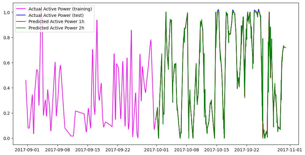

%matplotlib inline

plt.figure(figsize=(12, 6))
# plt.plot(val_df_nf["y"].tail(20), label="Actual Active Power (training)", color='magenta')
# plt.plot(test_df_nf["y"].head(20), label="Actual Active Power (test)", color='blue')
plt.plot(val_df_nf["y"].tail(50), label="Actual Active Power (training)", color='magenta')
plt.plot(test_df_nf["y"].head(100), label="Actual Active Power (test)", color='blue')
plt.plot(preds_df['1h']['NHITS'].head(100), label="Predicted Active Power 1h", color='red')
plt.plot(preds_df['2h']['NHITS'].head(100), label="Predicted Active Power 2h", color='green')
plt.plot(preds_df['3h']['NHITS'].head(100), label="Predicted Active Power 3h", color='orange')

plt.legend(fontsize='small')
plt.show();plt.close()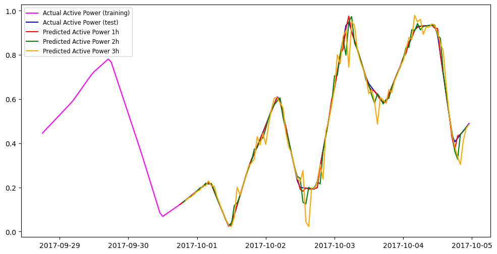

MAE computation

We will next compute the MAE for each of the predictions in the dictionary. The trickiest part here is to ensure that the predictions are aligned with the test set.

from sklearn.metrics import mean_absolute_error

test_df_nf.index.min(), test_df_nf.index.max()

(Timestamp('2017-09-30 20:00:00'), Timestamp('2017-10-30 23:00:00'))

test_df_nf['Wind_speed_tower']

time
2017-09-30 20:00:00    0.135542
2017-09-30 21:00:00    0.128765
2017-09-30 22:00:00    0.108434
2017-09-30 23:00:00    0.105422
2017-10-01 00:00:00    0.165663
                         ...   
2017-10-30 19:00:00    0.443524
2017-10-30 20:00:00    0.475904
2017-10-30 21:00:00    0.490964
2017-10-30 22:00:00    0.476657
2017-10-30 23:00:00    0.463102
Name: Wind_speed_tower, Length: 724, dtype: float64

mae1h_df = preds_df['1h'].copy()[2:][['NHITS']]
mae1h_df

	NHITS
ds
2017-09-30 20:00:00	0.143255
2017-09-30 21:00:00	0.152949
2017-09-30 22:00:00	0.161771
2017-09-30 23:00:00	0.174423
2017-10-01 00:00:00	0.184522
...	...
2017-10-30 19:00:00	0.721681
2017-10-30 20:00:00	0.721199
2017-10-30 21:00:00	0.720640
2017-10-30 22:00:00	0.719790
2017-10-30 23:00:00	0.719289

724 rows × 1 columns

We need to add the exogenous variables as they were used by the scaler.

mae1h_df.insert(0, 'Wind_speed_tower', test_df_nf['Wind_speed_tower'].values)
mae1h_df

	Wind_speed_tower	NHITS
ds
2017-09-30 20:00:00	0.135542	0.143255
2017-09-30 21:00:00	0.128765	0.152949
2017-09-30 22:00:00	0.108434	0.161771
2017-09-30 23:00:00	0.105422	0.174423
2017-10-01 00:00:00	0.165663	0.184522
...	...	...
2017-10-30 19:00:00	0.443524	0.721681
2017-10-30 20:00:00	0.475904	0.721199
2017-10-30 21:00:00	0.490964	0.720640
2017-10-30 22:00:00	0.476657	0.719790
2017-10-30 23:00:00	0.463102	0.719289

724 rows × 2 columns

# mae1h_df.columns = ["Wind_speed_tower", "Active_Power"]
mean_absolute_error(scaler.inverse_transform(mae1h_df)[:,1], test_df_original["Active_Power"])

0.006674091426698358

Mae for 2h preddictions

mae2h_df = preds_df['2h'].copy()[1:][:-1][['NHITS']]
mae2h_df

	NHITS
ds
2017-09-30 20:00:00	0.142033
2017-09-30 21:00:00	0.152502
2017-09-30 22:00:00	0.161576
2017-09-30 23:00:00	0.169637
2017-10-01 00:00:00	0.184456
...	...
2017-10-30 19:00:00	0.721748
2017-10-30 20:00:00	0.720069
2017-10-30 21:00:00	0.720531
2017-10-30 22:00:00	0.720106
2017-10-30 23:00:00	0.719239

724 rows × 1 columns

mae2h_df.insert(0, 'Wind_speed_tower', test_df_nf['Wind_speed_tower'].values)
mae2h_df

	Wind_speed_tower	NHITS
ds
2017-09-30 20:00:00	0.135542	0.142033
2017-09-30 21:00:00	0.128765	0.152502
2017-09-30 22:00:00	0.108434	0.161576
2017-09-30 23:00:00	0.105422	0.169637
2017-10-01 00:00:00	0.165663	0.184456
...	...	...
2017-10-30 19:00:00	0.443524	0.721748
2017-10-30 20:00:00	0.475904	0.720069
2017-10-30 21:00:00	0.490964	0.720531
2017-10-30 22:00:00	0.476657	0.720106
2017-10-30 23:00:00	0.463102	0.719239

724 rows × 2 columns

# mae1h_df.columns = ["Wind_speed_tower", "Active_Power"]
mean_absolute_error(scaler.inverse_transform(mae2h_df)[:,1], test_df_original["Active_Power"])

0.02290388513652618

Mae for 3h preddictions

mae3h_df = preds_df['3h'].copy()[:-2][['NHITS']]
mae3h_df

	NHITS
ds
2017-09-30 20:00:00	0.142487
2017-09-30 21:00:00	0.152598
2017-09-30 22:00:00	0.158074
2017-09-30 23:00:00	0.172433
2017-10-01 00:00:00	0.181613
...	...
2017-10-30 19:00:00	0.721319
2017-10-30 20:00:00	0.721116
2017-10-30 21:00:00	0.717298
2017-10-30 22:00:00	0.719902
2017-10-30 23:00:00	0.719717

724 rows × 1 columns

mae3h_df.insert(0, 'Wind_speed_tower', test_df_nf['Wind_speed_tower'].values)
mae3h_df

	Wind_speed_tower	NHITS
ds
2017-09-30 20:00:00	0.135542	0.142487
2017-09-30 21:00:00	0.128765	0.152598
2017-09-30 22:00:00	0.108434	0.158074
2017-09-30 23:00:00	0.105422	0.172433
2017-10-01 00:00:00	0.165663	0.181613
...	...	...
2017-10-30 19:00:00	0.443524	0.721319
2017-10-30 20:00:00	0.475904	0.721116
2017-10-30 21:00:00	0.490964	0.717298
2017-10-30 22:00:00	0.476657	0.719902
2017-10-30 23:00:00	0.463102	0.719717

724 rows × 2 columns

mean_absolute_error(scaler.inverse_transform(mae3h_df)[:,1], test_df_original["Active_Power"])

0.04667031221239267